vLLM-Omni Squeezes 172% More Audio Out of Four Speech Models

vLLM-Omni just published a detailed engineering breakdown of how it optimized TTS inference for four production-grade speech models: Qwen3-TTS, VoxCPM2, Higgs Audio V3, and Fish Speech S2 Pro. The headline numbers are striking , up to 172% more audio throughput and P99 latency cut nearly in half , but the real story is the methodology: there is no universal recipe. Every model got a different fix, because every model had a different bottleneck.

TTS is not just a slow LLM

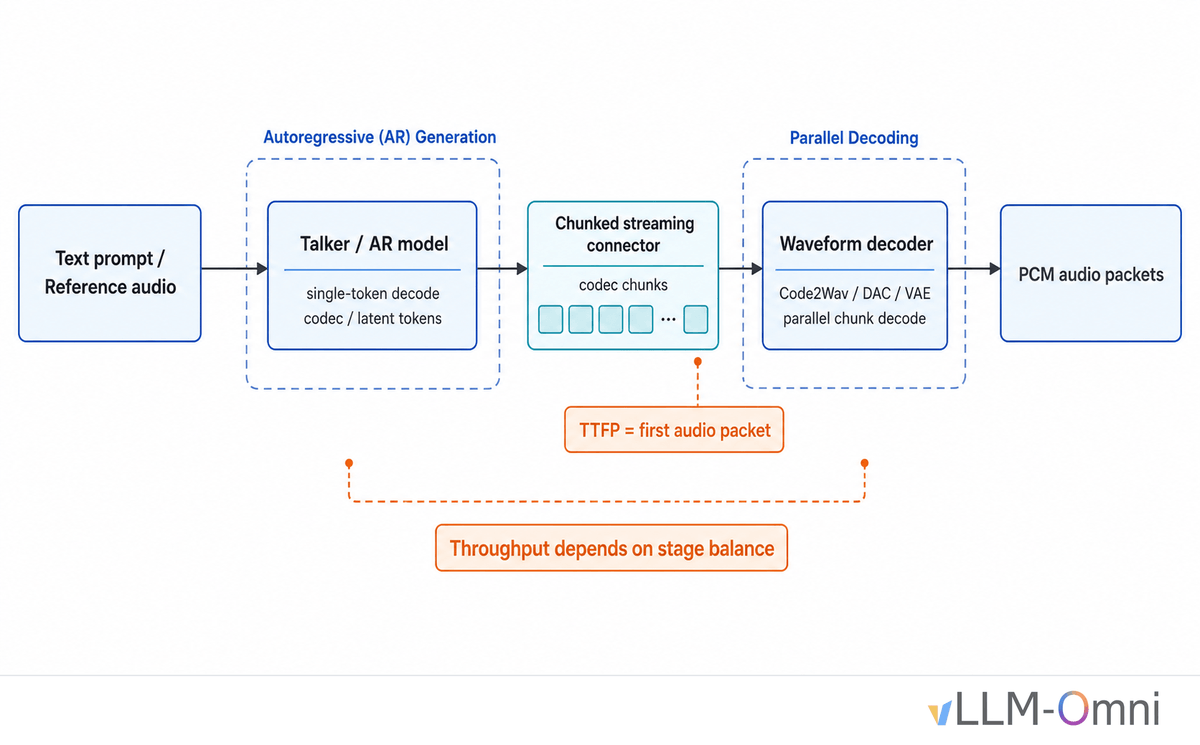
Most LLM serving optimizations assume a single autoregressive decode loop. TTS systems have at least two stages: a Talker that predicts codec tokens autoregressively, and a Code2Wav module that reconstructs waveform audio from those tokens. These stages have very different compute profiles , the Talker is latency-bound, while Code2Wav is throughput-bound. Treating them the same way means both suffer.

There are also constraints that simply do not exist in text generation. Users expect to hear the first audio packet within a few hundred milliseconds, and chunk size directly affects TTFP (Time To First Audio Packet). If chunks are too small, Code2Wav does not have enough context to keep audio continuous across chunk boundaries. If chunks are too large, first-packet latency becomes unacceptable. Throughput also matters for cost: how many concurrent streams a single GPU can sustain determines your deployment economics.

Four models, four levers

Here is a quick map of which technique was applied where and why:

• Qwen3-TTS , Python preprocessing overhead at high concurrency
• VoxCPM2 , Too many small compiled regions and underutilized GPU during diffusion decode
• Higgs Audio V3 , Multi-codebook state living in Python instead of on the GPU
• Fish Speech S2 Pro , Generic attention kernel carrying unnecessary overhead for a pure-decode shape

Qwen3-TTS: untangling the pipeline

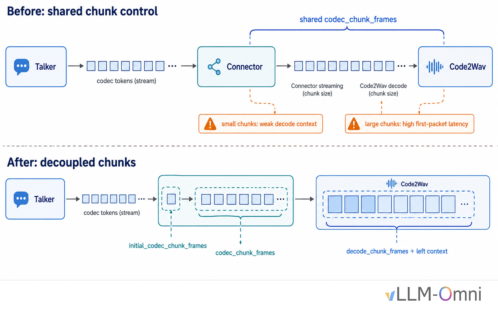
Qwen3-TTS has the most standard two-stage shape, making it a useful case study. The first problem was streaming. In the early implementation, connector streaming chunks and Code2Wav decode chunks were tied to the same parameter. If the connector sends very small chunks, Code2Wav sees very small decode chunks, hurting cross-chunk audio continuity. If you increase chunk size for quality, first-packet latency increases.

The fix was decoupling them into separate parameters: codec_chunk_frames controls the Talker-to-Code2Wav transfer cadence, while decode_chunk_frames and decode_left_context_frames control Code2Wav's internal decode window independently. A smaller initial_codec_chunk_frames lets Code2Wav start early, then later chunks return to the regular size.

The second problem was Python overhead at high concurrency. Each Qwen3-TTS Talker decode step needs request-level preprocessing: speaker embedding preparation, trailing_text maintenance, and input embedding construction. At c=64, every decode step loops over 64 requests, and Python-side loops plus tensor slicing become visible bottlenecks. GPU utilization told the same story , baseline average GPU utilization for Stage 0 was about 14%, meaning the GPU was mostly waiting on Python scheduling rather than doing compute.

The fix was batching. Speaker embeddings moved to GPU with cached mel basis buffers. The trailing_text sliding window switched from repeated tensor allocation to an offset-tracked buffer that only compacts when needed. Together with hot-path micro-optimizations (O(1) dict lookups replacing O(N²) list scans, precomputed codec-disallowed masks), the stacked result on H20×2 at c=64 was:

• Audio throughput: 26.55 → 42.88 audio-s/s (+61.5%)
• Median E2E latency: 9,654ms → 5,699ms (−41%)
• P99 E2E latency: 17,686ms → 8,956ms (−49.4%)

VoxCPM2: why per-layer compile wasn't enough

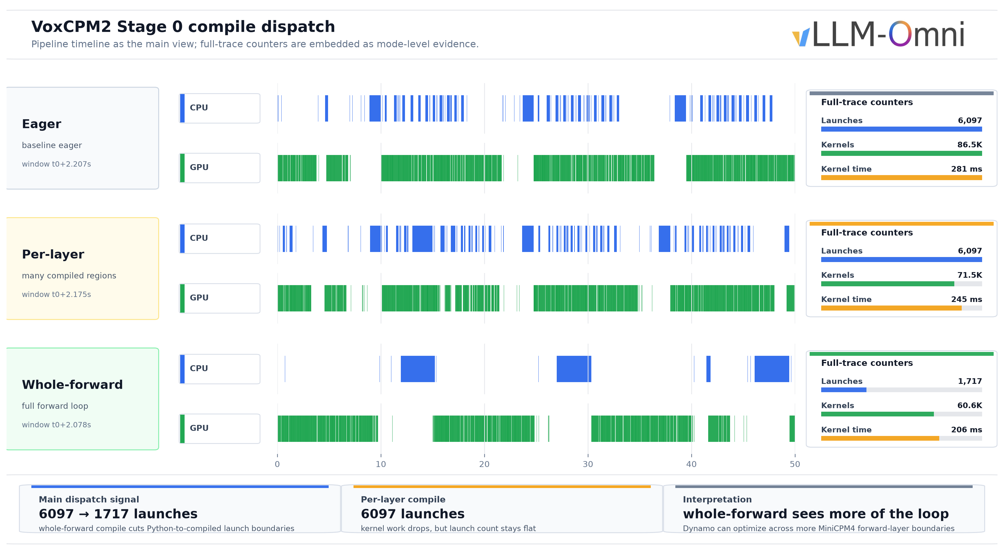
VoxCPM2 uses a diffusion-autoregressive hybrid design built around a 28-layer MiniCPM4 backbone, followed by a Conditional Flow Matching (CFM) diffusion decoder called LocDiT that iteratively denoises latent audio representations. The first instinct was to compile each layer's MLP and output projection separately , 56 compiled regions with fullgraph=True. The problem is that Dynamo cannot optimize across compiled-region boundaries. Each boundary adds a Python-to-compiled-to-Python transition, and 56 regions mean many transitions per decode step.

Wrapping the entire Model.forward in torch.compile with fullgraph=False was the key step. cudaLaunchKernel count dropped by about 71%, kernel events by about 30%, and kernel time by about 27%. The whole-forward approach lets Dynamo see the full 28-layer loop while still allowing PagedAttention's graph breaks to fall back to eager.

The second bottleneck was the CFM/LocDiT decode tail. At high concurrency, each request runs its own tiny diffusion batch (typically B=2 under classifier-free guidance), far too small to fill the GPU. The solution is to batch the CFM/LocDiT decode tail across requests: collect outputs from multiple requests, run the diffusion forward pass once as a batch, then scatter results back to request state. The result on H20×1 at c=64:

• Request throughput: 4.19 → 10.83 req/s (+158.8%)
• Audio throughput: 12.16 → 33.07 audio-s/s (+172%)

There was also a subtle synchronization bug: calling .item() on GPU tensors inside the Euler integration loop for CFM forces a GPU-to-CPU sync. The original path did this four times per diffusion step. With 10 timesteps and roughly 60 decode steps, one request could trigger around 2,400 synchronizations. Replacing .item() with GPU-side .copy_() broadcasting eliminates all of them.

Higgs Audio V3: moving state off the CPU

Higgs Audio V3 uses a MusicGen-style delay pattern across 8 codebooks, meaning each decode step must track which codebook each request is currently on, plus EOC (end-of-codes) countdown, generation-done flags, and related metadata. The main throughput gain came from moving this per-request Python dict state machine into GPU-resident batched tensors, reducing Python per-request loops, reducing device-to-host synchronization, and moving sampling and state update logic onto the batched GPU hot path. The result was a 2.7× speedup over baseline on a single H20 at c=16.

CUDA Graph support required an additional workaround. The Talker uses a boolean mask to select which requests are in decode state, but CUDA Graph capture requires fixed input/output shapes. A mask whose output shape depends on runtime data breaks that requirement. The fix: force the graph path to use a uniform single-token decode batch where the mask is always all-True, making the selection a no-op with a stable shape.

Fish Speech S2 Pro: a kernel built for one job

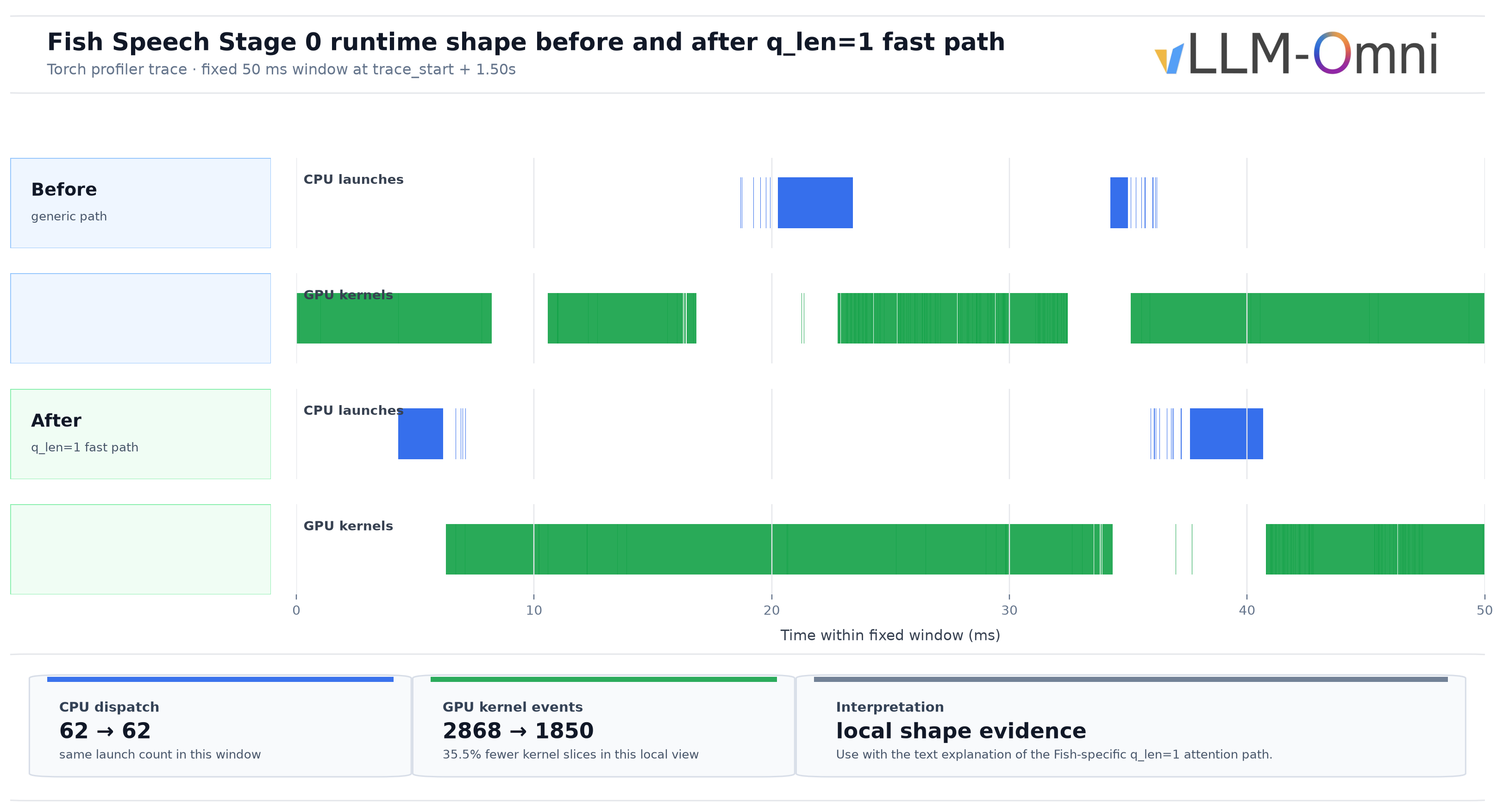
Fish Speech S2 Pro uses a Dual-AR architecture (slow_ar for semantic tokens, Fast AR for residual codebooks) trained on over 10 million hours of audio. Unlike the other three models, its bottleneck was not Python overhead , it was the GPU itself. Generic paged/varlen attention carries shape checks and branches for prefill, chunked prefill, decode, and other model shapes. For Fish's pure decode shape, that flexibility is overhead.

The team wrote a Fish-specific Triton kernel for SlowAR decode attention. It handles only q_len=1, fp16/bf16, head_dim=128, block size 16, and Fish's GQA layout. Short sequences (up to 1024 tokens) use a single-pass online softmax; longer sequences use a split-partial-combine path to handle reference audio with long context. For sequences that don't meet the shape constraints, it falls back to the original attention path.

What's available and how to use it

vLLM-Omni 0.20.0 refreshes the serving and runtime stack for large-scale omni workloads and improves diffusion model performance, quantization, and hardware readiness across CUDA, ROCm, MUSA, NPU, and XPU backends. All four TTS models are available in the vLLM-Omni GitHub repo as open-source. TTS deployment recipes are published at recipes.vllm.ai, including Qwen3-TTS and Higgs-Audio v3.

Serving a model is a single command:

vllm serve Qwen/Qwen3-TTS-12Hz-1.7B-CustomVoice \
  --deploy-config vllm_omni/deploy/qwen3_tts.yaml \
  --omni \
  --port 8091 \
  --trust-remote-code

The optimizations are most relevant if you are running TTS at scale , multiple concurrent streams per GPU, streaming output with tight first-audio latency budgets, or voice cloning workloads where preprocessing overhead compounds across hundreds of decode steps. If you're running single-request offline inference, the gains are smaller. For questions and contributions, the team is active in the #sig-omni channel on vLLM Slack.

The broader implication

The deeper lesson here is about serving infrastructure assumptions. The complexity of multi-stage multimodal model structures introduces substantial challenges for efficient serving, and existing frameworks are typically specialized for a single generation paradigm. The vLLM-Omni team's approach , profile each model independently, identify the actual bottleneck, and apply a targeted fix , is a template for anyone building production TTS infrastructure. The same GPU that looked 14% utilized under a naive serving setup can deliver 2–3× more audio throughput with the right lever pulled.