After a short family break, I am excited to be back and catching up on a busy few weeks of open-weight LLM releases. The thing that stood out to me is how much newer architectures are focused on long-context efficiency.

As reasoning models and agent workflows keep more tokens around (for longer), KV-cache size, memory traffic, and attention cost quickly become the main constraints, and LLM developers are adding a growing number of architecture tricks to reduce those costs.

The main examples I want to look at are KV sharing and per-layer embeddings in Gemma 4, layer-wise attention budgeting in Laguna XS.2, compressed convolutional attention in ZAYA1-8B, and mHC plus compressed attention in DeepSeek V4.

Most of these changes look like small tweaks in my architecture diagrams, but some of them are quite intricate design changes that are worth a more detailed discussion.

Note that this article is about architecture designs, so I will mostly skip dataset mixtures, training schedules, post-training details, RL recipes, benchmark tables, and product comparisons. Even with that narrower scope, there is a lot to cover. And, like always, the article turned out longer than I expected, so I will keep the focus on what changes inside the transformer block, residual stream, KV cache, or attention computation.

Please also note that I am only covering those topics that are interesting (new) design choices and that I haven’t covered elsewhere, yet. This list includes:

1. KV sharing and per-layer embeddings in Gemma 4

2. Compressed convolutional attention in ZAYA1

3. Attention budgeting in Laguna XS.2

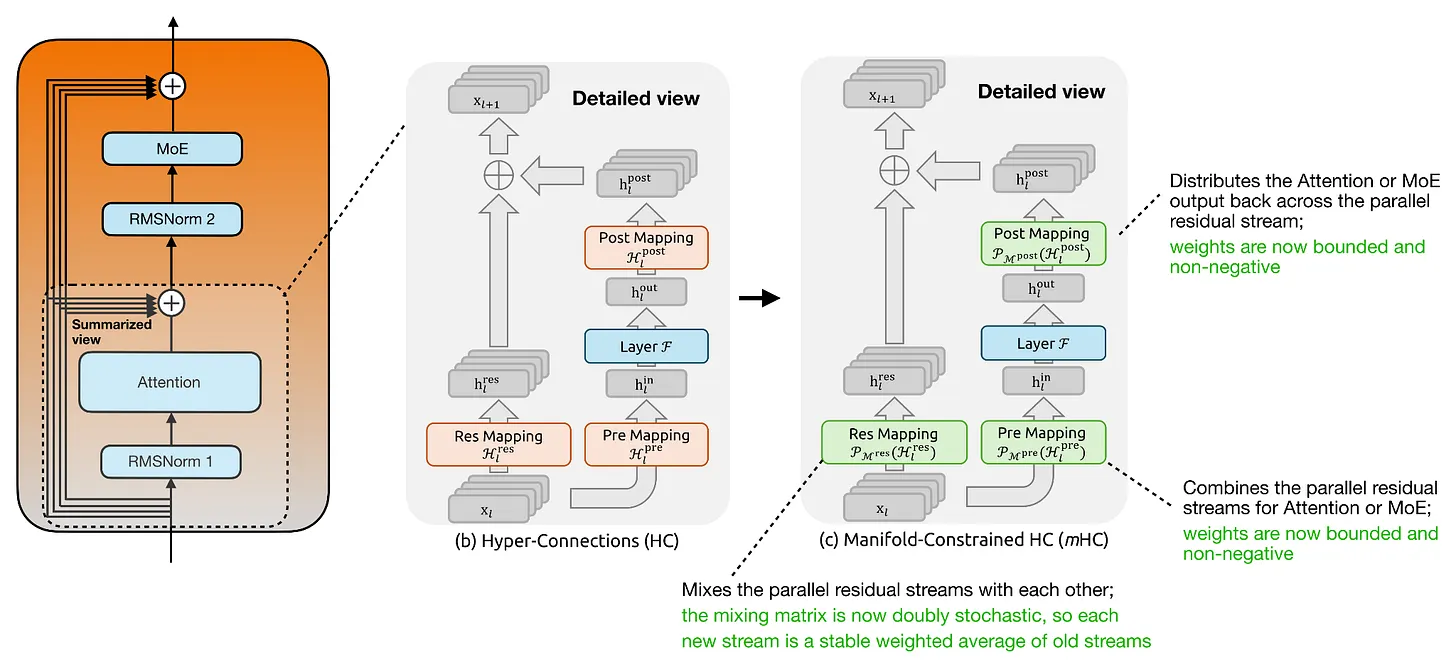
4. mHC and compressed attention in DeepSeek V4

Previous Topics

Before getting into the new parts, here are the two previous articles I will refer back to. The first one gives a broader architecture background on recent MoE models, routed experts, active parameters, and model-size comparisons. The second one covers the attention background that comes up repeatedly below, including MHA, MQA, GQA, MLA, sliding-window attention, sparse attention, and hybrid attention designs.

I also turned several of these explanations into short, standalone tutorial pages in the LLM Architecture Gallery. For example, readers can find compact explainers for GQA, MLA, sliding-window attention, DeepSeek Sparse Attention, MoE routing, and other concepts linked from the corresponding model cards and concept labels.

1. Reusing KV Tensors Across Layers to Shrink the Cache (Gemma 4)

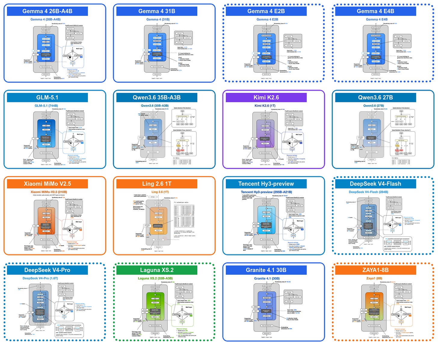
For this tour of architecture advances and tweaks, we will go back to the beginning of April when Google released their new open-weight Gemma 4 suite of models. They come in 3 broad categories:

• the Gemma 4 E2B and E4B models for mobile and small, local (embedded) devices (aka IoT),

• the Gemma 4 26B mixture-of-experts (MoE) model, optimized for efficient local inference,

• and the Gemma 4 31B dense model, for maximum quality and more convenient post-training (since MoEs are trickier to work with)

The first small architecture tweak in the E2B and E4B variants is that they adopt a shared KV cache scheme, where later layers reuse key-value states from earlier layers to reduce long-context memory and compute.

This KV-sharing was not invented by Gemma 4. For instance, see Brandon et al., “Reducing Transformer Key-Value Cache Size with Cross-Layer Attention” (NeurIPS 2024). But it’s the first popular architecture where I saw this concept applied. (Cross-layer attention is not to be confused with cross-attention.)

Before explaining KV-sharing further, let’s briefly talk about the motivation. As I wrote and talked about in recent months, one of the main recent themes in LLM architecture design is KV cache size reduction. In turn, the motivation behind KV cache size reduction is to reduce the required memory, which allows us to work with longer contexts, which is especially relevant in the age of reasoning models and agents. For more background on KV caching, see my “Understanding and Coding the KV Cache in LLMs from Scratch” article:

Practically all of the popular attention variants I described in my previous A Visual Guide to Attention Variants in Modern LLMs article are designed to reduce the KV cache size:

To pick a classic example (that Gemma 4 still uses): Grouped Query Attention (GQA) already shares key-value (KV) heads across different query heads to reduce the KV cache size, as illustrated in the figure below.

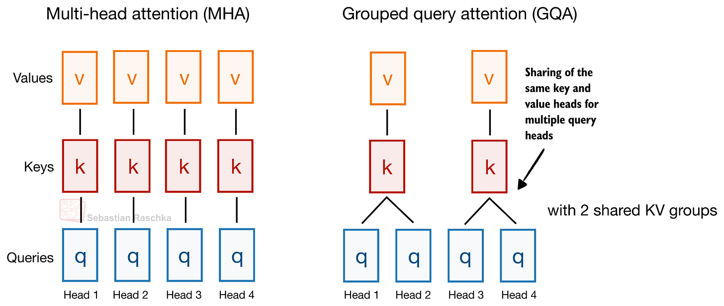
As mentioned before, Gemma 4 uses GQA. However, in addition to the KV sharing among queries as part of GQA, Gemma 4 also shares KV projections across different layers instead of computing it as part of the attention module in each layer. This KV-sharing scheme, also called cross-layer attention, is illustrated in the figure below.

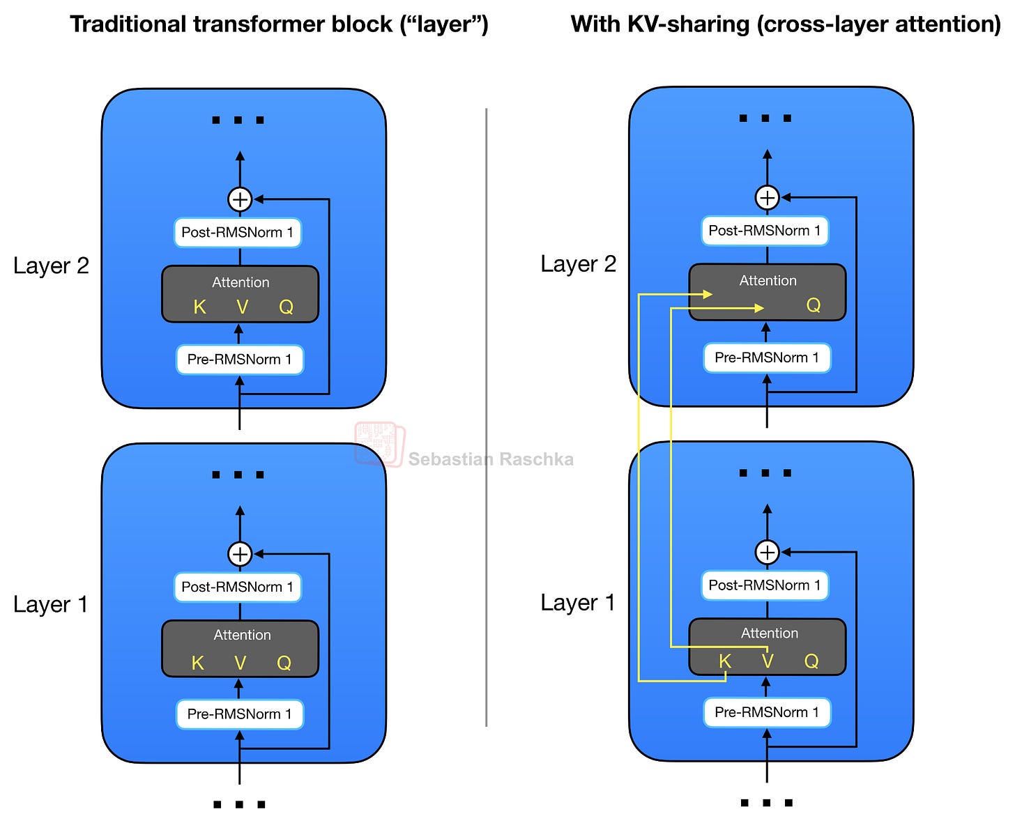
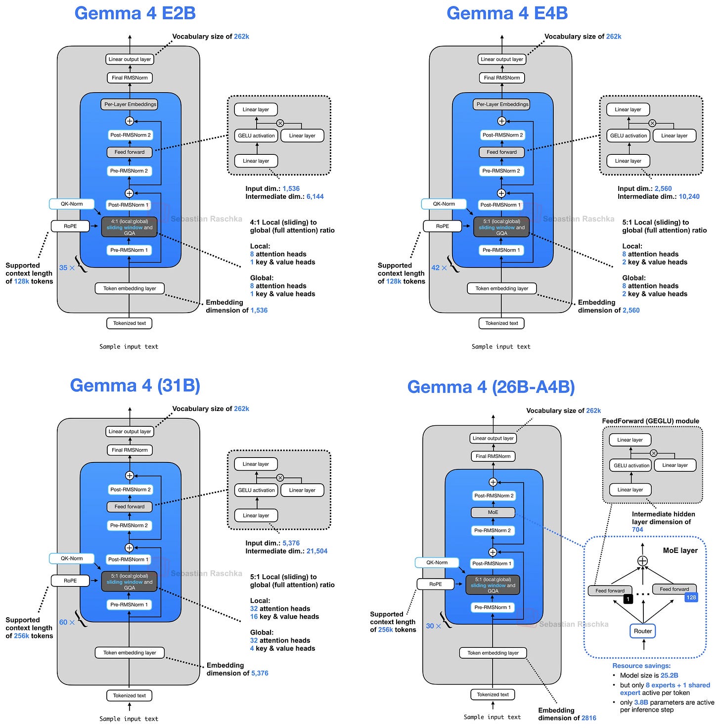
As briefly hinted at in the architecture overview in Figure 2, Gemma 4 E2B uses regular GQA and sliding window attention in a 4:1 pattern. (More precisely, Gemma 4 E2B uses MQA, which is the one-KV-head special case of GQA).

In the case of GQA (or MQA), the KV-sharing works like this. Later layers no longer compute their own key and value projections but reuse the KV tensors from the most recent earlier non-shared layer of the same attention type. In other words, sliding-window layers share KV with a previous sliding-window layer. Full-attention layers share KV with a previous full-attention layer. The layers still compute their own query projections, so each layer can form its own attention pattern, but the expensive and memory-heavy KV cache is reused across several layers.

For example, Gemma 4 E2B has 35 transformer layers, but only the first 15 compute their own KV projections; the final 20 layers reuse KV tensors from the most recent earlier non-shared layer of the same attention type. Similarly, Gemma 4 E4B has 42 layers, with 24 layers computing their own KV and the final 18 layers sharing them.

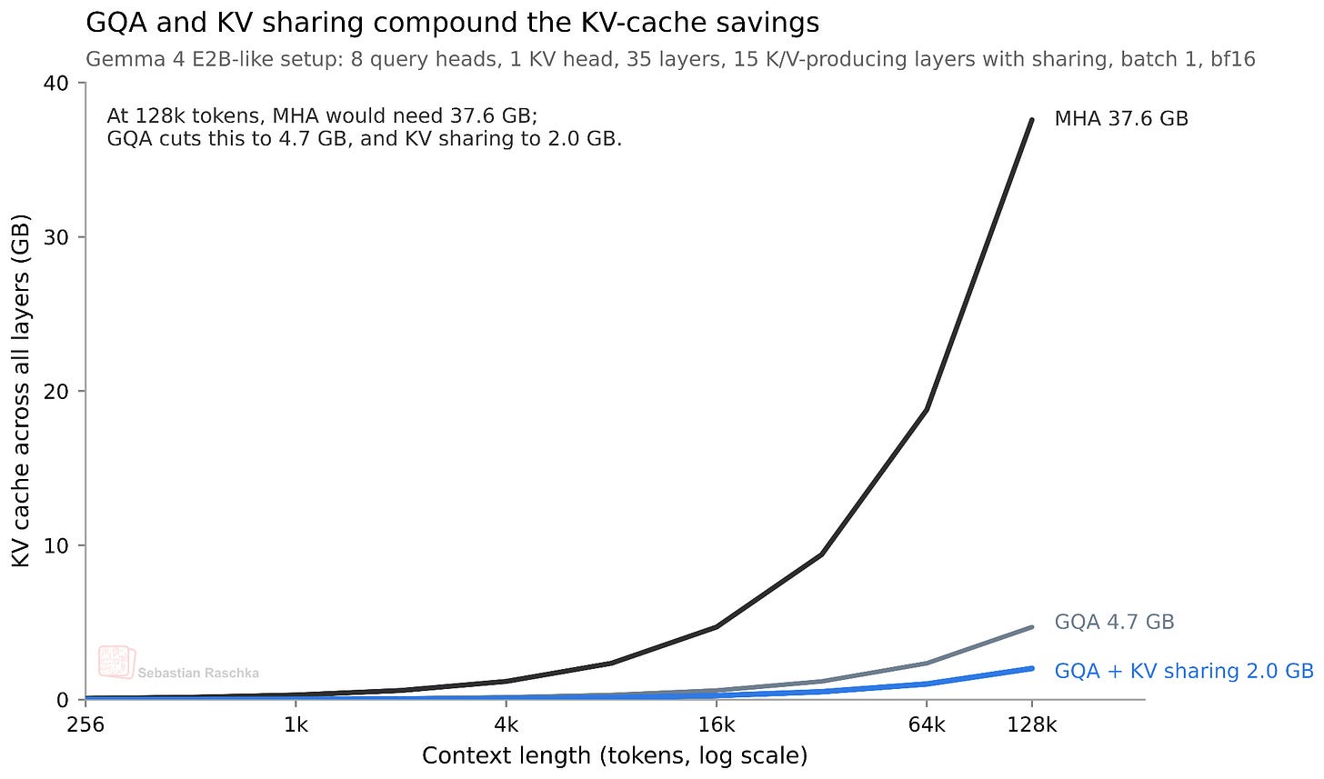
How much does this actually save? Since we share roughly half of the KVs across layers, we save approximately half of the KV cache size. For the smallest E2B model, this results in a 2.7 GB saving (at bfloat16 precision) in long 128K contexts, as shown below. (For the E4B variant, this saves about 6 GB at 128K.)

The downside of KV-sharing is, of course, that it’s an “approximation” of the real thing. Or, more precisely, it reduces model capacity. However, according to the cross-layer attention paper, the impact can be minimal (for small models that were tested).

2. Per-Layer Embeddings and “Effective” Size (Gemma 4 E2B/E4B)

The Gemma 4 E2B and E4B variants include a second efficiency-oriented design choice called per-layer embeddings (PLE). This is separate from the KV-sharing scheme above.

KV sharing reduces the KV cache. PLE is instead about parameter efficiency, where it lets the small Gemma 4 models use more token-specific information without making the main transformer stack as expensive as a dense model with the same total parameter count.

For instance, the “E” in Gemma 4 E2B and E4B stands for “effective”. Concretely, Gemma 4 E2B is listed as 2.3B effective parameters, or 5.1B parameters when the embeddings are counted. (Similarly, Gemma 4 E4B is listed as 4.5B effective parameters, or 8B parameters with embeddings).

In short, in the “E” models, the main transformer-stack compute is closer to the smaller number, while the larger number includes the additional embedding-table layers. (For an illustration of how embedding layers work, see my “